A journey into classical mechanics and the surprising importance of initial velocity
The Problem with Existing Simulations
While preparing a lesson on Atwood machines, I found myself frustrated with the online simulations available. They were fine for demonstrating the basic concept—two masses, a pulley, gravity at work—but they all shared a critical limitation: none of them allowed you to set an initial velocity.
This might seem like a minor omission, but it obscures a fundamental aspect of physics that I wanted my students to understand: the direction of acceleration and the direction of motion are not always the same.
In an Atwood machine where m₂ > m₁, the acceleration is always in one direction (clockwise, with m₂ descending). But if you give the system an initial velocity in the opposite direction, the lighter mass will initially move down even though the acceleration is pulling it up. The system will slow down, stop, and then reverse direction—just like throwing a ball upward despite gravity pulling it down.
This is a beautiful demonstration of the independence of acceleration and velocity, but I couldn’t find a simulation that showed it. So I decided to build one myself.
The Physics Behind the Machine
The Atwood machine is elegantly simple in its mechanics. Two masses, m₁ and m₂, connected by an inextensible string over a frictionless pulley. The physics gives us two key equations:
Acceleration
\(a = \frac{g(m_2 - m_1)}{m_1 + m_2}\)
This tells us something important: the acceleration depends only on the difference in masses, not their absolute values. If m₁ = m₂, then a = 0, and the system moves at constant velocity—a perfect demonstration of Newton’s first law.
Tension
\(T = \frac{2m_1 m_2 g}{m_1 + m_2}\)
The tension is always between m₁g and m₂g, approaching the geometric mean of the two weights. This intermediate value reflects the compromise between the two masses pulling in opposite directions.
Sign Convention
I chose to define clockwise rotation as positive: when m₂ descends and m₁ ascends, velocities and accelerations are positive. This convention matters deeply when we introduce initial velocity—a negative initial velocity means the system starts moving counterclockwise, opposite to its natural acceleration.
The Crucial Role of Initial Velocity
Here’s where it gets interesting. Consider an Atwood machine with m₁ = 2 kg and m₂ = 3 kg:
- Acceleration: a = 9.8(3-2)/(2+3) = 1.96 m/s² (clockwise, always)
- Initial velocity: Let’s say v₀ = -3 m/s (counterclockwise)
What happens?
- At t = 0: The system is moving counterclockwise at 3 m/s (m₁ descending, m₂ ascending)
- Immediately: Acceleration opposes motion, beginning to slow it down
- At t ≈ 1.53 s: The system momentarily stops (v = 0)
- After t > 1.53 s: The system reverses direction and accelerates clockwise
The masses change direction mid-flight! The acceleration never changes sign, but the velocity does. This is kinematics in action, and it’s exactly the kind of conceptual understanding I wanted to visualize.
Building the Simulation
The simulation needed to be more than just functional—it needed to be educational. Here’s what I prioritized:
1. Visual Clarity
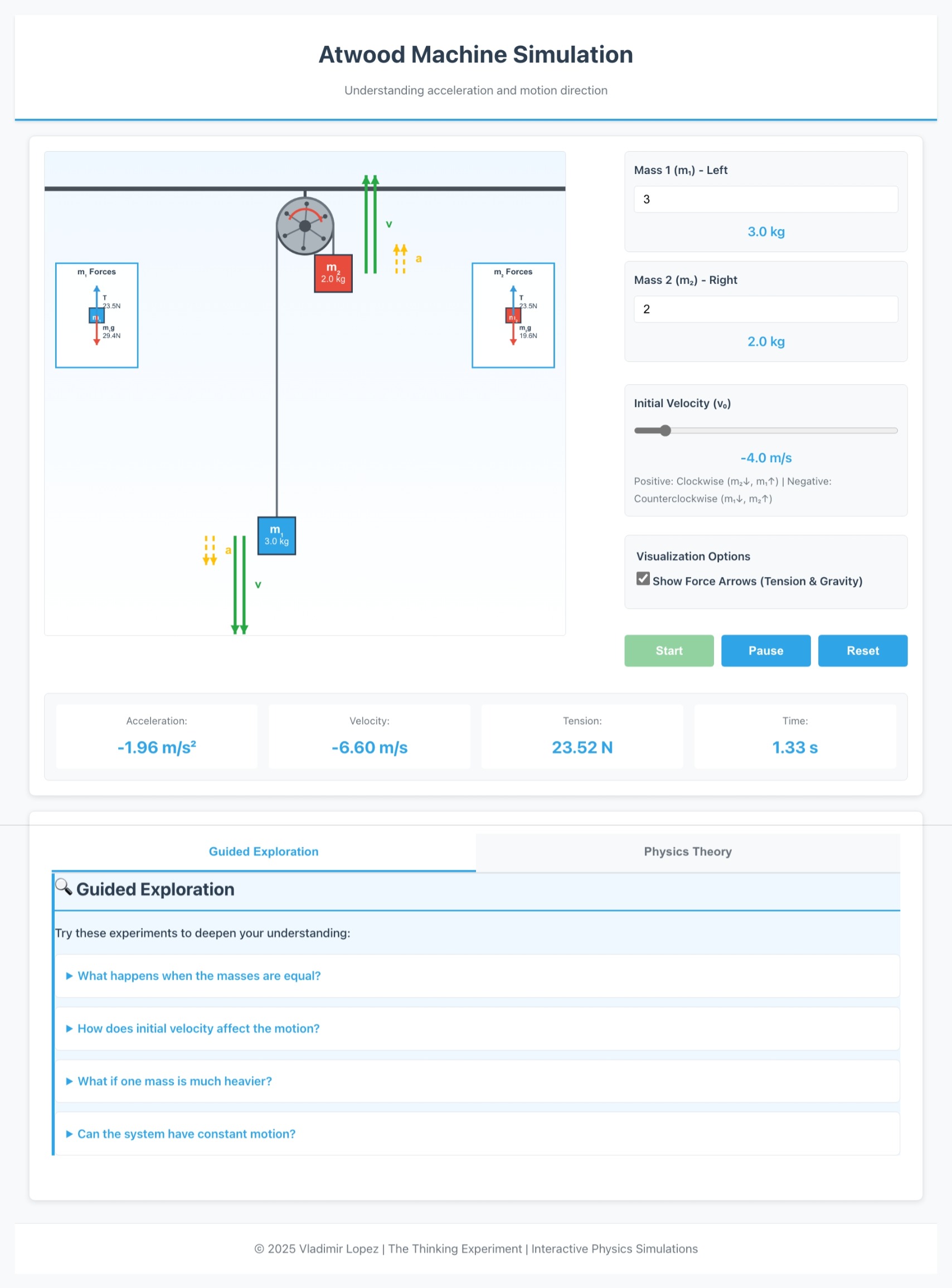
The masses are color-coded (blue for m₁, red for m₂) and labeled clearly. The ropes are drawn with proper geometry: vertical lines from each mass to the tangent points on the pulley, then an arc over the top. This matches how we draw Atwood machines in textbooks.
2. Dynamic Vector Visualization
Each mass has two sets of arrows beside it: - Green solid arrows for velocity (v) - Yellow dashed arrows for acceleration (a)
These arrows scale with the magnitude of the quantities and point in the correct direction: - Up (negative) when the mass is moving or accelerating upward - Down (positive) when the mass is moving or accelerating downward
As the simulation runs, you can watch the velocity arrows grow and shrink, reverse direction, while the acceleration arrows remain constant (for fixed masses). It’s mesmerizing.
3. Real-Time Data Display
The simulation continuously updates: - Current acceleration (a) - Current velocity (v) - Tension in the string (F_T) - Elapsed time (t)
This numerical feedback complements the visual representation, helping students connect the abstract equations to the concrete motion.
4. Interactive Controls
Students can adjust: - Mass 1: 0.1 to 10 kg - Mass 2: 0.1 to 10 kg
- Initial Velocity: -5 to +5 m/s
The ability to set initial velocity is the key differentiator. Want to see constant motion? Set m₁ = m₂ and any v₀ ≠ 0. Want to see direction reversal? Set unequal masses with v₀ opposite to the acceleration. Want to understand equilibrium? Set everything to zero.
5. Educational Context
Below the simulation, I included theoretical background: what an Atwood machine is, the key equations, and practical applications. This isn’t just a toy—it’s a teaching tool.
Technical Implementation
The simulation is built entirely in HTML5 Canvas with vanilla JavaScript—no frameworks, no dependencies beyond MathJax for equation rendering. The physics engine uses simple Euler integration:
// Update physics each frame
this.velocity += this.acceleration * this.dt;
this.position2 += this.velocity * this.dt;
this.time += this.dt;
With dt = 0.008 seconds and pixelsPerMeter = 25, the motion is smooth and realistic. The masses stay on screen, the vectors update in real time, and the equations remain accurate throughout.
The code is structured around an AtwoodMachine class that handles: - Physics calculations - Canvas rendering - Animation loop - User input
Clean separation of concerns makes the code maintainable and extensible.
What I Learned
Building this simulation reinforced several lessons:
Teaching tools should highlight what’s hard to see: The relationship between acceleration and velocity is subtle. Making it visual makes it understandable.
Details matter: Arrow direction, sign conventions, label placement—these small choices affect pedagogical clarity.
Interactivity beats passivity: Letting students explore parameter space themselves is more powerful than showing them one example.
Simple can be powerful: You don’t need a physics engine or 3D graphics. Canvas and careful math are enough.
Try It Yourself
Open the simulation in a new tab
Try this experiment: 1. Set m₁ = 2 kg, m₂ = 3 kg 2. Set initial velocity to -3 m/s 3. Click Start 4. Watch the green velocity arrows
Notice how they start pointing up (counterclockwise motion), shrink as the system decelerates, disappear momentarily at the turning point, then reappear pointing down as the system accelerates in its natural direction. The yellow acceleration arrows never change—they point down for m₂ and up for m₁ throughout, because the acceleration is constant.
That’s the insight I wanted to convey. Motion and acceleration are related, but they’re not the same. And sometimes, you need to see it to believe it.
Closing Thoughts
The Atwood machine is over 200 years old, but it still has lessons to teach. By adding one feature—initial velocity control—we unlock a richer understanding of kinematics. The system doesn’t always move the way you expect, and that’s exactly why it’s worth studying.
If you’re a teacher, I hope this simulation helps your students. If you’re a student, I hope it deepens your intuition. And if you’re just curious about physics, I hope it reminds you that even the simplest systems can surprise us.
Physics is beautiful because it’s universal. The same equations that govern an Atwood machine govern the motion of planets, pendulums, and projectiles. Understanding one helps you understand them all.
Now go play with the simulation. Set some wild initial conditions. See what happens. That’s how we learn.
Vladimir Lopez
The Thinking Experiment
October 24, 2025